GloVe
In this section of the tutorial we will discuss the intuition behind the GloVe embeddings and how they are created.
Word2Vec
Before we discuss GloVe vectors, we should briefly discuss word2vec, as both combine the principle of distributional semantics (you can tell a word’s meaning by the words surrounding it) and unsupervised machine learning. The intuition behind word2vec is the following: Instead of implementing a count-based method directly, let us train a classifier instead that will predict a word from its k-window context (or the other way around). We are not actually interested in the classifier itself, instead we use its internal layer as our embeddings.
Essentially, how this works in practice is that we randomly assign each word a vector and randomly assign vectors to each words’ contexts. The size of the context is defined by the k-window we use. We then train a classifier to either predict the word from the context (CBOW) or the context from the word (skip-gram). These are the two architectures of word2vec. This is done via a three layer neural network. The middle hidden layer contains weights which are continuously updated during training. After the model is done training, we throw out the classifier and keep those weights as our word vectors. This is the very abridged version of word2vec.
GloVe
GloVe was introduced by Pennigton et. al 2014 and it combines the insights of word2vec, that local context is a powerful predictor, with global co-occurence statistics. Word2vec exclusively relies on local context and its model iterates over the data multiple times until it converges, which can be quite costly with large corpora. So even though word2vec iterates over the entire corpus, it only ever consideres local information. This means, for example, that if there are words which are quite frequent globally, word2vec may overestimate their importance locally. Here global means the entire corpus, whereas local refers to the k-window.
In order to overcome these types of issues, GloVe utilizes both the local context, as well as global co-occurances. It does this by utilizing a pre-computed global co-occurence matrix. Assume a corpus of 50,000 unique words. The co-occurrence matrix will be a 50,000 X 50,000 matrix. Every row denotes a word and every column in a row denotes how many times that word co-occurs with another word in the context k-window. It’s important to understand, that the global co-occurence does not refer to how many times the word occurs in the corpus in general, but rather, how many times they co-occur in a k-window. Now that we have these raw co-occurences, we can use that to compute a probability matrix, which will give us the probablity of word X co-occuring with word Y in ths corpus:
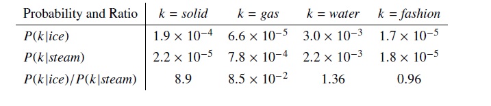 Example of a co-occurence probability matrix from Pennigton et al. (2014, 3)
Why is this useful? Well, to translate an example from Pennigton et al. (2014, 3), we can use this to find relationships between words. For example, take i = ice and j = steam. We can learn something about their relationship by studying the the “ratio of their co-occurrence probabilities with various probe words” (Pennigton et al. 2014, 3). So, if we take a third probe word say k = solid we can divide the probability of ice given solid, P_ik, by the probability of steam given solid, P_jk. If the result of that division is a large number, we can assume that solid is relevant to ice but not relevant to steam. If the result is a small number, we can assume that solid is relevant to steam, but not to ice. If the result approximates 1, it can be assumed to be irrelevant to either words. The assumption that we can leverage global co-occurence in this way is really the basis of the GloVe model.
A problem here is that some words will rarely or even never co-occur. So there will be quite a few zero entries in our matrix. Even those entries that are non-zero but very small, will create some undesired noise in the data. To deal with this, the GloVe team proposed the following cost function:
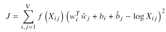
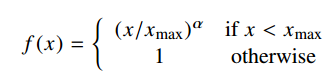
Where X_ij is the frequency of two words co-occuring. f(X_ij) is a continuous function that vanishes if X=0, and has a hard threshhold as to not overweigh very frequent co-occurences:
The model generates two sets of word vectors. If the co-occurence matrix is symmetric (which it is in the original implementation), both vectors should be equivalent, differing only because they were randomly initialized. The final word vector is the sum of those two vectors.
In other regards, GloVe functions similarly to word2vec. Except for predicting a word from its context, the GloVe model is trained to predict the co-occurrence matrix.
Making your own GloVe style embeddings
Let us now move on the next part of the tutorial, where we learn how to use the authors original implementation to make our own vectors. Next Page
References
Jeffrey Pennington, Richard Socher, and Christopher D. Manning. 2014. GloVe: Global Vectors for Word Representation. Mikolov, Tomas (2013). “Distributed representations of words and phrases and their compositionality”. Advances in Neural Information Processing Systems